Generating 2D Gating Hierarhcy from Clustered Cytometry Data

Our algorithm cluster-to-gates(C2G) can visualize a clustered cytometry data in 2D gating hierarchy. The overall input to C2G are two variables: "data" and "label". "data" is a N-by-M matrix where N is the number of cells and M is the number of markers. "label" is a N-by-1 matrix and this matrix represent which cluster each cell belongs to (0 for ungated cells). In this page, we will demonstrate how to use C2G to generate gating hierarchy on a simulated data and on a CyTOF dataset that are manually gated. The software and testing data can be downloaded here .

Initialization and load the simulated data
Visualize the simulated data and pre-clustered simulated data in 3D
Run the analysis on the simulated data
Load a moderate-sized CyTOF dataset with ~10,000 cells
Generate gating hierarchy for manually gated populations
Generate gating hierarchy for K-means defined populations (K=10)
Apply C2G to large CyTOF dataset with ~140,000 cells
Reference

Initialization and load the simulated data

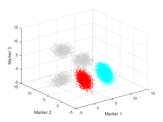
This simulated data set contains 20000 cells, which consists of 5 populations.Two of the populations are considered as target and labeled as 1 and 2. The cells in other populations are labeled 0 which means "unlabeled". A visualization of the original data is also shown in the following sections.

addpath('src')
addpath('libs')
load('testdata/simulated.mat','data','label');
markernames ={'Marker 1','Marker 2','Marker 3'};
fprintf('Size of "data" is %d-by-%d\n',size(data));
fprintf('Size of "label" is %d-by-%d\n',size(label));

Size of "data" is 20000-by-3
Size of "label" is 20000-by-1

Visualize the simulated data and pre-clustered simulated data in 3D

In real application, this section is not necessay.

col = [0.8 0.8 0.8;hsv(length(unique(label))-1)];
figure('Position',[680 478 560 420]);
scatter3(data(:,1),data(:,2),data(:,3),1,col(label+1,:));
xlabel('Marker 1')
ylabel('Marker 2')
zlabel('Marker 3')
axis([-5 15 -5 15 -5 15]);

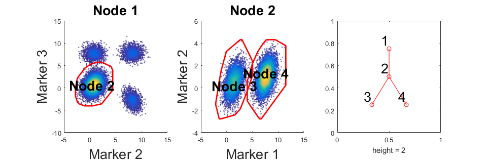
Run the analysis on the simulated data

This section performs the analysis on the simulated data. If your data has no "unlabeled" cells, precluster step can be skipped. If you skip precluster, the second and third parameter in function "C2G" should be the same.

% Precluster the simulated data
rng(9464);
preclustered_label = cluster_ungated(data,label);

% Call main part of the program and return a object m that store the
% results.
m = C2G(data,preclustered_label,label,'markernames',markernames);
% Draw the obtained gating hierarchy
m.view_gates(data,markernames,'n_lines',1,'onepanel',true);
% Show statistics
outtable = m.show_f_score(label);

Step:  0	[100%]
[Selected] marker pair Marker 2 and Marker 3
Population	Gate	    TP	    FP	    FN	F-score
         1	   1	  5411	 14589	     0	  0.426
         2	   1	  9166	 10834	     0	  0.629
Normalized Mutual Information = 0.321
Step:  1	[100%]
[Selected] marker pair Marker 1 and Marker 2
Population	Gate	    TP	    FP	    FN	F-score
         1	   2	  5411	  9183	     0	  0.541
         2	   2	  9166	  5428	     0	  0.772
Normalized Mutual Information = 0.736
Step:  2	[100%]No further separation. Node 3 is gate for cell population 1
Step:  3	[100%]No further separation. Node 4 is gate for cell population 2
Population	Gate	    TP	    FP	    FN	F-score
         1	   3	  5411	    18	     0	  0.998
         2	   4	  9166	     1	     0	  1.000
Normalized Mutual Information = 0.996

Load a moderate-sized CyTOF dataset with ~10,000 cells

This is a dataset about T cell signaling (Krishnaswamy et al, Science, 2014). It can be downloaded from here. This section will load multiple fcs files. Each fcs file correspond to one cell population manually gated by the authors. C2G will automatically generate cell labels based on fsc files. FCS files are store in the "testdata" folder. "CD4_Effmen.fcs", "CD4_naive.fcs", and "CD8_naive.fcs" are cells of target populations (manually defined) and "ctr.fcs" contain all cells. In this example, we only use surface protein markers.

clear
close all
addpath('src')
addpath('libs')
fdname = 'testdata';
[ori_data,ori_l,ori_markers]=load_mul_fcs(fdname,'ctr.fcs');

surface_idx = [3 4 6 8 9 11 12 13 22 24 25 27];
data = ori_data(:,surface_idx);
markers = ori_markers(surface_idx);
n_markers = length(markers);

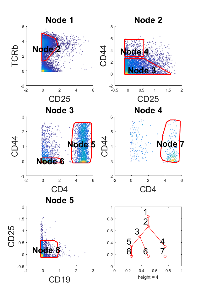
Generate gating hierarchy for manually gated populations

In this section, we'll use the data loaded from previous section and treat the three manually defined cell populations as target populations. Here, number of "unlabeled" cells is around two-fold of cells in target populations. The results (the table below) show that C2G can capture manually defined populations at very high accuracy.

% Precluster the ungated cells
rng(9464)
label = cluster_ungated(data,ori_l);
% Perform the anlysis
m_ori = C2G(data,label,ori_l,'markernames',markers);
% Visualize the results
m_ori.view_gates(data,markers,'n_lines',3,'ignore_small',0,'onepanel',true);
m_ori.show_f_score(ori_l);

Population	Gate	    TP	    FP	    FN	F-score
         1	   7	   216	    13	     8	  0.954
         2	   8	  2267	    30	    78	  0.977
         3	   6	   488	    46	    37	  0.922
Normalized Mutual Information = 0.893

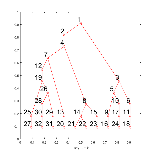
Generate gating hierarchy for K-means defined populations (K=10)

In this section, we will use the same CyTOF data used in previous section. The cell labels are defined by k-means algorithm where k equal to 10. All of the 10 clusters will be considered as target populations, in other words,there're no "unlabeled" cells.

rng(9464)
km_l = kmeans(data,10);
new_km_l = km_l; % Since all populiations is known, no need to pre-cluster
% Perform the anlysis
m_km = C2G(data,km_l,km_l,'markernames',markers);
% Visualize the results
m_km.view_gates(data,markers,'n_lines',4,'ignore_small',300);
m_km.show_f_score(km_l);

Population	Gate	    TP	    FP	    FN	F-score
         1	  27	   746	   155	    42	  0.883
         2	  16	   798	   139	   115	  0.863
         3	  32	  1204	   176	    85	  0.902
         4	  24	  1853	   243	   277	  0.877
         5	  31	  1418	   161	    74	  0.923
         6	  18	  1163	   165	   208	  0.862
         7	  21	   714	    27	    38	  0.956
         8	  20	   138	    12	    18	  0.902
         9	  22	   609	    38	    46	  0.935
        10	  23	   192	    15	    26	  0.904
Normalized Mutual Information = 0.780

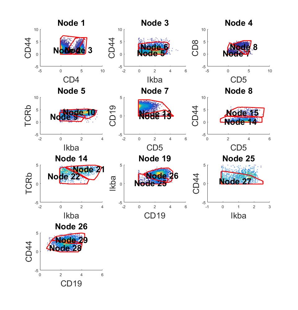
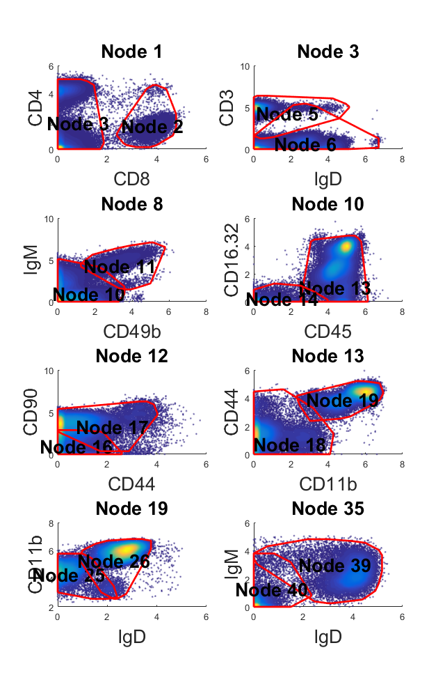
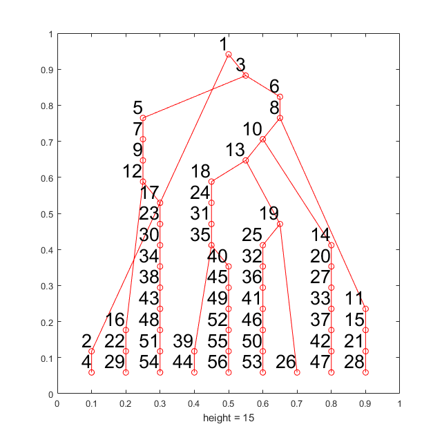
Apply C2G to large CyTOF dataset with ~140,000 cells

This is a larger CyTOF dataset with 140k cells and 21 protein markers (Spitzer, Matthew H., et al, Science, 2015 ). This data can be download for free from here. (The dataset is hosted on Cytobank and you need to register to download it) This dataset is clustered by k-means where k equal to 10. All of the 10 k-means defined clusters are treated as target populations. This part will take around 10 minutes on a desktop.

[ori_data, marker] = readfcs_v2('testdata/bigdata/TIN_BLD1_Untreated_Day3.fcs');
% Transform the CyTOF
data = flow_arcsinh(ori_data,5);
% Select protein markers
marker_idx = [10,16,17,18,19,21,22,24,29,31,32,33,39,40,41,46,47,49,50,51,52];
d = data(marker_idx,:)';
rng(9464);
label = kmeans(d,10);
% Perform the anlysis
tic;m = C2G(d, label, label,'markernames',marker(marker_idx));toc;
% Visualize the results
w = warning ('off','all');
m.view_gates(d,marker(marker_idx),'ignore_small',3000,'n_lines',4);
warning(w);
m.show_f_score(label);

Population	Gate	    TP	    FP	    FN	F-score
         1	  29	 15390	   534	  1172	  0.947
         2	  47	  6683	   255	   544	  0.944
         3	  26	 10863	 14070	  1338	  0.585
         4	  44	 19313	    85	   822	  0.977
         5	  53	  9833	   301	  1164	  0.931
         6	  26	 13421	 11512	   784	  0.686
         7	   4	 13324	    35	   442	  0.982
         8	  54	 29331	   833	  1526	  0.961
         9	  28	  6993	   460	   398	  0.942
        10	  56	  7804	   218	   726	  0.943
Normalized Mutual Information = 0.859

Reference

Krishnaswamy, Smita, Matthew H. Spitzer, Michael Mingueneau, Sean C. Bendall, Oren Litvin, Erica Stone, Dana Pe’er, and Garry P. Nolan. "Conditional density-based analysis of T cell signaling in single-cell data." Science 346, no. 6213 (2014): 1250689.

Spitzer, Matthew H., Pier Federico Gherardini, Gabriela K. Fragiadakis, Nupur Bhattacharya, Robert T. Yuan, Andrew N. Hotson, Rachel Finck et al. "An interactive reference framework for modeling a dynamic immune system." Science 349, no. 6244 (2015): 1259425.